Using DQN to solve the Banana environment from ML-Agents - Part (1)

This is an Part-1 of an accompanying post for the submission of the Project 1: navigation from the Udacity Deep Reinforcement Learning Nanodegree, which consisted on building a DQN-based agent to navigate and collect bananas from the Banana Collector environment from Unity ML-Agents.

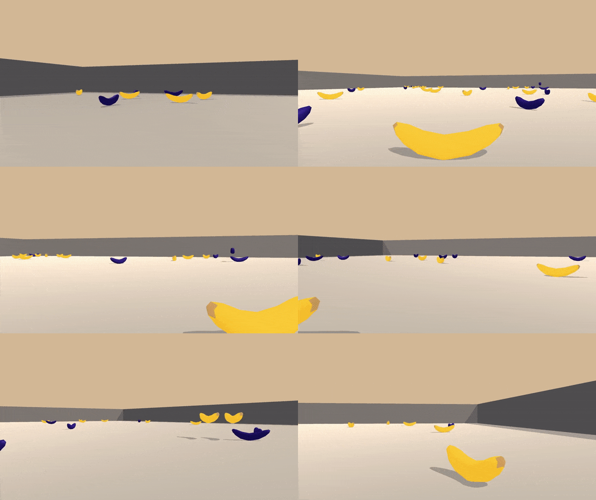
The following are the topics to be covered in this post:

1. Description of the Banana Collector Environment.
2. Setting up the dependencies to run the accompanying code.
3. An overview of the DQN algorithm.

1. Description of the Banana Collector Environment

The environment chosen for the project was a modified version of the Banana Collector Environment from the Unity ML-Agents toolkit. The original version can be found here, and our version consists of a custom build provided by Udacity with the following description:

• A single agent that can move in a planar arena, with observations given by a set of distance-based sensors and some intrinsic measurements, and actions consisting of 4 discrete commands.
• A set of NPCs consisting of bananas of two categories: yellow bananas, which give the agent a reward of +1, and purple bananas, which give the agent a reward of -1.
• The task is episodic, with a maximum of 300 steps per episode.

1.1 Agent observations

The observations the agent gets from the environment come from the agent's linear velocity in the plane (2 entries), and a set of 7 ray perceptions. These ray perceptions consist of rays shot in certain fixed directions from the agent. Each of these perceptions returns a vector of 5 entries each, whose values are explained below:

• The first 4 entries consist of a one-hot encoding of the type of object the ray hit, and these could either be a yellow banana, a purple banana, a wall or nothing at all.
• The last entry consist of the percent of the ray length at which the object was found. If no object is found at least at this maximum length, then the 4th entry is set to 1, and this entry is set to 0.0.

Below there are two separate cases that show the ray-perceptions. The first one to the left shows all rays reaching at least one object (either purple banana, yellow banana or a wall) and also the 7 sensor readings in array form (see the encodings in the 4 first entries do not contain the none found case). The second one to the right shows all but one ray reaching an object and also the 7 sensor readings in array form (see the encodings in the 4 first entries do include the none found case for the 4th perception).

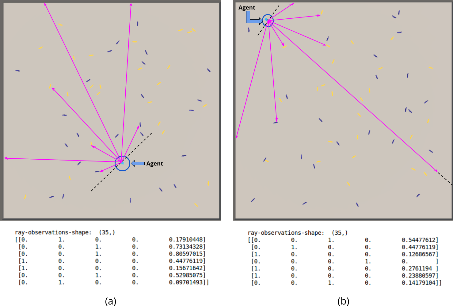
All these measurements account for an observation consisting of a vector with 37 elements. This vector observation will be the representation of the state of the agent in the environment that we will use as input to the Q-network, which will be discussed later.

Note

This representation is applicable only to our custom build (provided by Udacity), as the original Banana Collector from ML-Agents consists of a vector observation of 53 entries. The rays in the original environment give extra information about the current state of the agent (the agent in the original environment can shoot and be shot), which give 2 extra measurements, and the rays give also information about neighbouring agents (2 extra measurements per ray).

If curious, you can take a look at the C# implementation in the UnitySDK folder of the ML-Agents repository. See the 'CollectObservations' method (shown below) in the BananaAgent.cs file. This is helpfull in case you want to create a variation of the environment for other purposes other than this project.

    public override void CollectObservations()
    {
        if (useVectorObs)
        {
            float rayDistance = 50f;
            float[] rayAngles = { 20f, 90f, 160f, 45f, 135f, 70f, 110f };
            string[] detectableObjects = { "banana", "agent", "wall", "badBanana", "frozenAgent" };
            AddVectorObs(rayPer.Perceive(rayDistance, rayAngles, detectableObjects, 0f, 0f));
            Vector3 localVelocity = transform.InverseTransformDirection(agentRb.velocity);
            AddVectorObs(localVelocity.x);
            AddVectorObs(localVelocity.z);
            AddVectorObs(System.Convert.ToInt32(frozen));
            AddVectorObs(System.Convert.ToInt32(shoot));
        }
    }

1.2 Agent actions

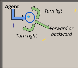
The actions that the agent can take consist of 4 discrete actions that serve as commands for the movement of the agent in the plane. The indices for each of these actions are the following :

• Action 0: Move forward.
• Action 1: Move backward.
• Action 2: Turn left.
• Action 3: Turn right.

Figure 3 shows these four actions that conform the discrete action space of the agent.

Note

These actions are applicable again only for our custom build, as the original environment from ML-Agents has even more actions, using action tables (newer API). This newer API accepts in most of the cases a tuple or list for the actions, with each entry corresponding to a specific action table (a nested set of actions) that the agent can take. For example, for the original banana collector environment the actions passed should be:

# actions are of the form: [actInTable1, actInTable2, actInTable3, actInTable4]

# move forward
action = [ 1, 0, 0, 0 ]
# move backward
action = [ 2, 0, 0, 0 ]
# mode sideways left
action = [ 0, 1, 0, 0 ]
# mode sideways right
action = [ 0, 2, 0, 0 ]
# turn left
action = [ 0, 0, 1, 0 ]
# turn right
action = [ 0, 0, 2, 0 ]

1.3 Environment dynamics and rewards

The agent spawns randomly in the plane of the arena, which is limited by walls. Upon contact with a banana (either yellow or purple) the agents receives the appropriate reward (+1 or -1 depending on the banana). The task is considered solved once the agent can consistently get an awerage reward of +13 over 100 episodes.

2. Accompanying code and setup

The code for our submission is hosted on github. The README.md file already contains the instruction of how to setup the environment, but we repeat them here for completeness (and to save you a tab in your browser 😆).

2.1 Custom environment build

The environment provided is a custom build of the ml-agents Banana Collector environment, with the features described in the earlier section. The environment is provided as an executable which we can download from the links below according to our platform:

Platform	Link
Linux	Link
Mac OSX	Link
Windows (32-bit)	Link
Windows (64-bit)	Link

Keep the .zip file where you downloaded it for now. We will later explain where to extract its contents when finishing the setup.

Note

The executables provided are compatible only with an older version of the ML-Agents toolkit (version 0.4.0). The setup below will take care of this, but keep this in mind if you want to use the executable on your own.

2.2 Dependencies

As already mentioned, the environment provided is an instance of an ml-agents environment and as such it requires the appropriate ml-agents python API to be installed in order to interact with it. There are also some other dependencies, so to facilitate installation all this setup is done by installing the navigation package from the accompanying code, which we will discuss later. Also, there is no need to download the Unity Editor for this project (unless you want to do a custom build for your platform) because the builds for the appropriate platforms are already provided for us.

2.3 Downloading the accompanying code and finishing setup

• Grab the accompanying code from the github repo.

# clone the repo
git clone https://github.com/wpumacay/DeeprlND-projects
# go to the project1-navigation folder
cd DeeprlND-projects/project1-navigation

• (Suggested) Create an environment using a virtual environment manager like pipenv or conda.

# create a virtual env. using conda
conda create -n deeprl_navigation python=3.6
# activate the environment
source activate deeprl_navigation

• Install pytorch.

# Option 1: install pytorch (along with cuda). No torchvision, as we are not using it yet.
conda install pytorch cudatoolkit=9.0 -c pytorch
# Option 2: install using pip. No torchvision, as we are not using it yet.
pip install torch

• (Optional) Our implementation decouples the requirement of the function approximator (model) from the actual DQN core implementation, so we have also an implementation based on tensorflow in case you want to try that out.

# install tensorflow (1.12.0)
pip install tensorflow==1.12.0
# (Optional) In case you want to train it using a GPU
pip install tensorflow-gpu==1.12.0

• Install the navigation package using pip and the provided setup.py file (make sure you are in the folder where the setup.py file is located).

# install the navigation package and its dependencies using pip (dev mode to allow changes)
pip install -e .

• Uncompress the executable downloaded previously into the executables folder in the repository

cd executables/
# copy the executable into the executables folder in the repository
cp {PATH_TO_ZIPPED_EXECUTABLE}/Banana_Linux.zip ./
# unzip it
unzip Banana_Linux.zip

• (Update|Optional) If you want to use the tensorflow implementation, you might run into a little problem when setting up tensorflow. The issue comes from the unityagents pip package, because it requires us to install tensorflow 1.7.0, which overwrites the version we installed earlier. This will cause various problems even if we want to install again our tensorflow version. The workaround we found was to just install the unityagents package for version 0.4.0, which is provided by udacity in its repo, with a slight modification that removes the tensorflow 1.7.0 dependency. So, instead of using the installation steps from before, follow the steps from below.

# clone the udacity repo
git clone https://github.com/udacity/deep-reinforcement-learning.git

# go to the python folder of the repo
cd deep-reinforcement-learning/python

# remove the tensorflow dependency from the requirements.txt file with your favourite editor
vim requirements.txt # remove the tensorflow dependency

# install the unityagents package from this folder
pip install -e .

# install the requirements from our package
cd PATH_TO_OUR_PACKAGE
pip install -r requirements.txt

# install the appropriate tensorflow version after that
# either the gpu version
pip install tensorflow-gpu==1.12.0
# or the cpu version (it still can train with cpu in a moderate amount of time)
pip install tensorflow==1.12.0

3. An overview of the DQN algorithm

As mentioned in the title, our agent is based on the DQN agent introduced in the Human-level control through deep reinforcement learning paper by Mnih, et. al. We will give a brief description of the algorithm in this section, which is heavily based on Sutton and Barto's book. For completeness we will start with a brief introduction to reinforcement learning, and then give the full description of the DQN algorithm.

3.1 RL concepts

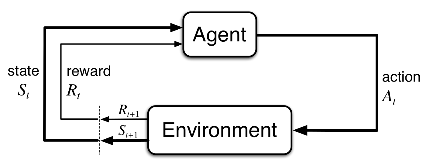
Reinforcement Learning (RL) is a learning approach in which an Agent learns by trial and error while interacting with an Environment. The core setup is shown in Figure 1, where we have an agent in a certain state \( S_{t} \) interacting with an environment by applying some action \( A_{t} \). Because of this interaction, the agent receives a reward \( R_{t+1} \) from the environment and it also ends up in a new state \( S_{t+1} \).

This can be further formalize using the framework of Markov Decision Proceses (MDPs). Using this framework we can define our RL problem as follows:

A Markov Decision Process (MDP) is defined as a tuple of the following components:

• A state space \( \mathbb{S} \) of configurations \( s_{t} \) for an agent.
• An action space \( \mathbb{A} \) of actions \( a_{t} \) that the agent can take in the environment.
• A transition model \( p(s',r | s,a) \) that defines the distribution of states that an agent can land on and rewards it can obtain \( (s',r) \) by taking an action \( a \) in a state \( s \).

The objective of the agent is to maximize the total sum of rewards that it can get from its interactions, and because the environment can potentially be stochastic (recall that the transition model defines a probability distribution) the objective is usually formulated as an expectation ( \( \mathbb{E} \) ) over the random variable defined by the total sum of rewards. Mathematically, this objective is described as follows.

\[ \mathbb{E} \left \{ r_{t+1} + r_{t+2} + r_{t+3} + \dots \right \} \]

Notice the expectation is over the sum of a sequence of rewards. This sequence comes from a trajectory (\( \tau \)) that the agent defines by interacting with the environment in a sequential manner.

\[ \tau = \left \{ (s_{0},a_{0},r_{1}),(s_{1},a_{1},r_{2}),\dots,(s_{t},a_{t},r_{t+1}),\dots \right \} \]

Tasks that always give finite-size trajectories can be defined as episodic, like in games, whereas tasks that go on forever are defined as continuous, like life itself (wait, I'm not elf 😨). The task we are dealing in this post is episodic, and the length of an episode (max. length of any trajectory) is 300 steps.

There is a slight addition to the objective defined earlier that is often used: the discount factor \( \gamma \). This factor tries to take into account the effect that a same ammount of reward in the far future should be less interesting to the agent than the same amount now (kind of like interest rates when dealing with money). We introduce this by multiplying each reward by a power of this factor to the number of steps into the future.

\[ \mathbb{E} \left \{ r_{t+1} + \gamma r_{t+2} + \gamma^{2} r_{t+3} + \dots \right \} \]

Sidenote: The most important reason we use discounting is for mathematical convenience, as it allows to keep our objective from exploding in the non-episodic case (to derive this, just replace each \( r_{t} \) for the maximum reward \( r_{max} \), and sum up the geometric series). There is another approach which deals with the undiscounted average reward setting. This approach leads to a different set of bellman equations from the ones that are normally studied, and therefore different algorithms.

A solution to the RL problem consists of a Policy \( \pi \), which is a mapping from the current state we are ( \( s_{t} \) ) to an appropriate action ( \( a_{t} \) ) from the action space. Such mapping is basically a function, and we can define it as follows:

A deterministic policy is a mapping \( \pi : \mathbb{S} \rightarrow \mathbb{A} \) that returns an action to take \( a_{t} \) from a given state \( s_{t} \).

\[ a_{t} = \pi(s_{t}) \]

We could also define an stochastic policy which, instead of returning an action \( a_{t} \) in a certain situation given by the state \( s_{t} \), it returns a distribution over all possible actions that can be taken in that situation \( a_{t} \sim \pi(.|s_{t}) \).

A stochastic policy is a mapping \( \pi : \mathbb{S} \times \mathbb{A} \rightarrow \mathbb{R} \) that returns a distribution over actions \( a_{t} \) to take from a given state \( s_{t} \).

\[ a_{t} \sim \pi(.|s_{t}) \]

Our objective can then be formulated as follows: find a policy \( \pi \) that maximizes the expected discounted sum of rewards.

\[ \max_{\pi} \mathbb{E}_{\pi} \left \{ r_{t+1} + \gamma r_{t+2} + \gamma^{2} r_{t+3} + \dots \right \} \]

To wrap up this section we will introduce three more concepts that we will use throughout the rest of this post: returns \( G \), state-value functions \( V(s) \) and action-value functions \( Q(s,a) \).

The return \( G_{t} \) is defined as the discounted sum of rewards obtained over a trajectory from time step \( t \) onwards.

\[ G_{t} = r_{t+1} + \gamma r_{t+2} + \gamma^{2} r_{t+3} + \dots = \sum_{k=0}^{\infty} \gamma^{k} r_{t+k+1} \]

By using the return we can write the objective of the agent in a more compact way, as follows:

\[ \max_{\pi} \mathbb{E}_{\pi} \left \{ G_{t} \right \} \]

The state-value function \( V_{\pi}(s) \) is defined as the expected return that an agent can get if it starts at state \( s_{t} = s \) and then follows policy \( \pi \) onwards.

\[ V_{\pi}(s) = \mathbb{E} \left \{ G_{t} | s_{t} = s; \pi \right \} \]

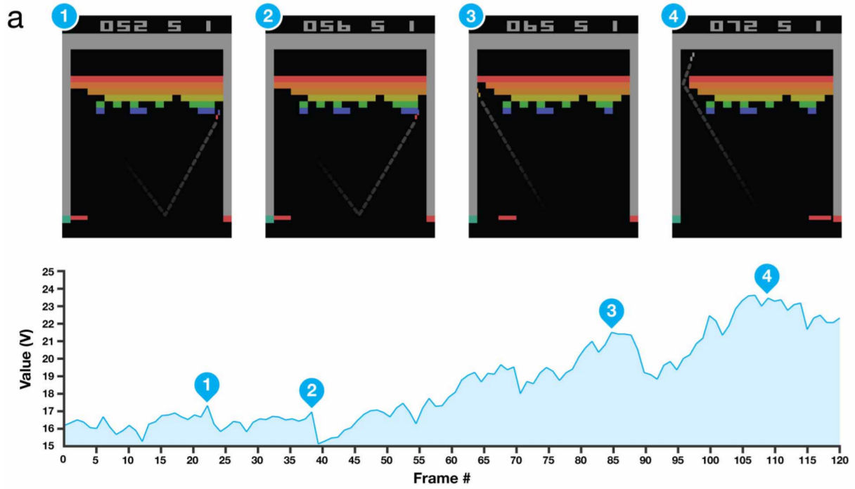
This function \( V_{\pi}(s) \) serves as a kind of intuition of how well a certain state is if we are following a specific policy. The figure below (taken from the DQN paper [2]) illustrates this more clearly with the game of breakout as an example. The agent's state-value function on the bottom part of the figure shows that in the state in which the agent makes a hole in the bricks its estimate of the value greatly increases (section labeled with 4) in the graph.

The action-value function \( Q_{\pi}(s,a) \) is defined as the expected return that an agent can get if it starts at state \( s_{t} = s \), takes an action \( a_{t} = a \) and then follows the policy \( \pi \) onwards.

\[ Q_{\pi}(s,a) = \mathbb{E} \left \{ G_{t} | s_{t} = s, a_{t} = a; \pi \right \} \]

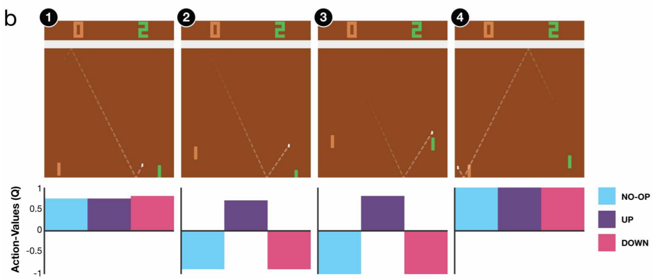
This function \( Q_{\pi}(s,a) \) serves also as a kind of intuition of how well a certain action is if we apply it in a certation state if we are following a specific policy. The figure below illustrates this more clearly (again, taken from the DQN paper [2]) with the game of pong as an example. The agent's action-value function tell us how well is a certain action in a certain situation, and as you can see in the states labeled with (2) and (3) the function estimates that action UP will give a greater return than the other two actions.

3.2 RL solution methods

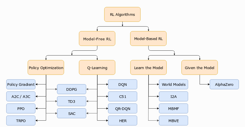
There are various methods that we can use to solve this problem. The figure below (from [3]) shows a taxonomy of the available approaches and methods within each approach. We will be following the Value-based approach, in which we will try to obtain the optimal action-value function \( Q^{\star} \).

Value based methods are based on the Bellman Equations, which specify what the optimal state-value and action-value functions should satisfy in order to be optimal. Below we show the Bellman Optimality Equation for \( Q^{\star} \), and the solution \( Q^{\star} \) of this equation is a fixed point that can be computed exactly using Dynamic Drogramming (if a model of the environment is known) or approximately with Monte Carlo and Temporal Difference methods (if no model of the environment is available).

\[ Q^{\star}(s,a) = \mathbb{E}_{(s,a,s',r)} \left \{ r + \gamma \max_{a'} Q^{\star}(s',a') \right \} \]

3.3 Tabular Q-learning

The method we will use is called Q-learning, which is a model-free method that recovers \( Q^{\star} \) from experiences using the following update rule:

\[ Q(s,a) := \overbrace{Q(s,a)}^{\text{Current estimate}} + \alpha ( \overbrace{r + \gamma \max_{a'} Q(s',a')}^{\text{"Better" estimate}} - Q(s,a) ) \]

This update rule is used in the tabular case, which is used when dealing with discrete state and action spaces. These cases allow to easily represent the action-value function in a table (numpy array or dictionary), and update each entry of this table separately.

For example, consider a simple MDP with \( \mathbb{S}=0,1\) and \( \mathbb{A}=0,1\). The action-value function could be represented with the following table.

State (s)	Action (a)	Q-value Q(s,a)
0	0	Q(0,0)
0	1	Q(0,1)
1	0	Q(1,0)
1	1	Q(1,1)

In python we could just use :

# define a Q-table initialized with zeros (using numpy)
import numpy as np
Q = np.zeros( (nStates, nActions), dtype = np.float32 )

# define a Q-table initialized with zeros (using dictionaries)
from collections import defaultdict
Q = defaultdict( lambda : np.zeros( nActions ) )

The Q-learning algorithm for the tabular case is shown below, and it basically consists of updating the estimate of the q-value \( Q(s,a) \) for the state-action pair \( (s,a) \) from another estimate of the true q-value of the optimal policy given by \( r + \gamma \max_{a'} Q(s',a') \) called the TD-Target.

Q-learning (off-policy TD control)

• Algorithm parameters: step size \( \alpha \in [0,1] \), small \( \epsilon \gt 0 \)

• Initialize q-table \( Q(s,a) \) for all \( s \in \mathbb{S}, a \in \mathbb{A} \)

• For each episode:

  • Sample initial state \( s_{0} \) from the starting distribution.
  • For each step \( t \) in the episode :
    • Select \( a_{t} \) from \( s_{t} \) using e-greedy from \( Q \)
    • Execute action \( a_{t} \) in the environment, and receive reward \( r_{t+1} \) and next state \( s_{t+1} \)
    • Update entry in q-table corresponding to \( (s,a) \):

\[ Q(s,a) := Q(s,a) + \alpha ( r + \gamma \max_{a'} Q(s',a') - Q(s,a) ) \]

In python we would have the following :

def qlearning( env, Q, eps, alpha, gamma, numEpisodes, maxStepsPerEpisode ) :
  """Run q-learning to estimate the optimal Q* for the given environment
  
  Args:
    env                 : environment to be solved
    Q                   : action value function represented as a table
    eps                 : epsilon value for e-greedy heuristic (exploration)
    alpha               : learning rate
    gamma               : discount factor
    numEpisodes         : number of episodes to run the algorithm
    maxStepsPerEpisode  : maximum number of steps in an episode
  """

  for iepisode in range( numEpisodes ) :
    # sample initial state from the starting distribution (given by env. impl.)
    _s = env.reset()

    for istep in range( maxStepsPerEpisode ) :
      # select action using e-greedy policy
      _a = np.random.randint( env.nA ) if np.random.random() < eps else np.argmax( Q[_s] )
      # execute action in the environment and receive reward and next state
      _snext, _r, _finished, _ = env.step( _a )
      # compute target to update
      if _finished :
        _tdTarget = _r
      else :
        _tdTarget = _r + gamma * np.max( Q[_snext] )
      # update entry for (_s,_a) using q-learning update rule
      Q[_s][_a] = Q[_s][_a] + alpha * ( _tdTarget - Q[_s][_a] )

      # cache info for next step
      _s = _snext

For further information about Q-learning you can check the resources from [4,5,6]

3.4 Function approximation

The tabular case provides a nice way to solve our problem, but at the cost of storing a big table with one entry per possible \( (s,a) \) pair. This is not scalable to larger state spaces, which is the case for continous spaces. One approach would be to discretize the state space into bins for various \( (s,a) \), treat each bin as an entry for the table and then solve as in the tabular case. However this is not practical for various reasons :

• As the discretization gets more precise we end up with more bins and our table explodes in size. This is an exponential explosion due to the curse of dimensionality.
• Each possible \( (s,a) \) is stored separately and updated separately, which doesn't take into account the fact that nearby \( (s,a) \) pairs should have similar \( Q(s,a) \) values. This means we are not generalizing our knowledge of one pair to nearby pairs.

To solve these issues we make use of function approximators like linear models, radial basis functions, neural networks, etc., which allow us to scale up to high dimensional spaces and "generalize" over these spaces.

Building on top of the previous Q-learning algorithm, we can write an algorithm to obtain the action-value function using function approximation. In this case we parametrize our action-value function as \( Q_{\theta}(s,a) \) where \( \theta \) are the parameters of the function approximator, e.g. the weights of a neural network. Recall from tabular Q-learning that the update rule tried to improve an estimate of a q-value \( Q(s,a) \) from another estimate \( r + \gamma \max_{a'} Q(s',a') \) which we called TD-target. This was necessary as we did not have a true value for the q-value at \( (s,a) \), so we had to use a guess.

Suppose we have access to the actual q-value for all \( (s,a) \) possible pairs. We could then use this true q-value and make our estimates become these true q-values. In the tabular case we could just replace these for each entry, and for the function approximation case we make something similar: What do we do if we have the true values (or labels) that our model has to give for some inputs?. Well, we just fit our model to the data like in supervised learning.

\[ \theta = \argmin_{\theta} \mathbb{E}_{(s,a) \sim D} \left \{ ( Q^{\star}(s,a) - Q_{\theta}(s,a) )^{2} \right \} \]

If our function approximator is differentiable we then could just use Gradient Descent to obtain the parameters \( \theta \) of our model:

\[ \theta := \theta - \frac{1}{2} \alpha \nabla_{\theta} \mathbb{E}_{(s,a) \sim D} \left \{ ( Q^{\star}(s,a) - Q_{\theta}(s,a) )^{2} \right \} \\ \rightarrow \theta := \theta - \frac{1}{2} \alpha \mathbb{E}_{(s,a) \sim D} \left \{ \nabla_{\theta}( Q^{\star}(s,a) - Q_{\theta}(s,a) )^{2} \right \} \\ \rightarrow \theta := \theta + \alpha \mathbb{E}_{(s,a) \sim D} \left \{ (Q^{\star}(s,a) - Q_{\theta}(s,a)) \nabla_{\theta}Q_{\theta}\vert_{(s,a)} \right \} \\ \]

Or, if using Stochastic Gradient Descent (SGD) :

\[ \theta := \theta + \alpha (Q^{\star}(s,a) - Q_{\theta}(s,a)) \nabla_{\theta}Q_{\theta}\vert_{(s,a)} \]

Unfortunately, we do not have an oracle that would tell us the true q-values for each possible \( (s,a) \) pair. Here we use a similar approach to tabular Q-learning, namely use an estimate of the true q-value to update our current estimate. This estimate of the true q-value was our TD-target, so we could just replace it in the SGD update rule derived before:

\[ \theta := \theta + \alpha (r + \gamma \max_{a'}Q_{\theta}(s',a') - Q_{\theta}(s,a)) \nabla_{\theta}Q_{\theta}\vert_{(s,a)} \]

This yields the following algorithm:

Action-Value function approximation

• Parameters: learning rate \( \alpha \in [0,1] \), small \( \epsilon \gt 0 \)

• Initialize a parametrized action-value function \( Q_{\theta} \)

• For each episode:

  • Sample initial state \( s_{0} \) from the starting distribution
  • For each step \( t \) in the episode :
    • Select \( a_{t} \) from \( s_{t} \) using e-greedy from \( Q_{\theta} \)
    • Execute action \( a_{t} \) in the environment, and receive reward \( r_{t+1} \) and next state \( s_{t+1} \)
    • If \( s' \) is terminal:
      • \( Q_{target} = r \)
    • Else:
      • \( Q_{target} = r + \gamma \max_{a'}Q_{\theta}(s',a') \)
    • Update parameters \( \theta \) using the following update rule :

\[ \theta := \theta + \alpha ( Q_{target} - Q_{\theta}(s_{t},a_{t}) ) \nabla_{\theta} Q_{\theta}\vert_{s=s_{t},a=a_{t}} \]

This algorithm forms the basis of the DQN agent, which adds various improvements on top of this base algorithm. These improvements help to stabilize learning as there are various issues when using the Vanilla version of this algorithm directly with a Deep Neural Network as a function approximator.

3.5 Deep Q-Learning

At last, this section will describe the Deep Q-Learning algorithm, which builds on top of the algorithm previously described.

3.5.1 End-to-end learning

A key issue we did not discussed in the previous section was how we used these function approximators, which is actually a similar story to the previous techniques used in Computer Vision before Deep Learning came back to life.

Usually when using a function approximator the inputs to this model are not direct raw sensory data, but some intermediate representation in the form of features. These features had to be carefully engineered for the specific task at hand (like in the case of Computer Vision). Fortunately, we can use Deep Learning to help us come with the right internal features required for the problem we are trying to solve, as shown in the image below.

Similarly, we can combine Deep Learning (as powerful function approximators) with Reinforcement Learning into a similar pipeline that would allow the agent learn the required representations to solve the task at hand.

However, unlike supervised learning, the RL setup forces us to deal with sequential data, which breaks the i.i.d. assumption (independent and identically distributed). This brings correlations in the data that break direct vanilla approaches (just replacing the function approximator with a deep network, and hoping for the best). Moreover, unlike the tabular setup, there are no convergence guarantees for our algorithms when using non-linear function approximators (see Chapter 11 in [1] for further info).

To solve part of these issues, the authors in [2] developed various improvements to the Vanilla setting that helped stabilize learning and break these annoying correlations: Experience Replay and Fixed Targets.

3.5.2 DQN: Experience Replay

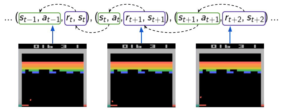
Experience replay is a mechanism introduced in [2] and it consists of Learning from past stored experiences during replay sessions. Basically, we remember our experiences in memory (called a replay buffer) and learn from them later. This allows us to make more efficient use of past experiences by not throwing away samples right away, and it also helps to break one type of correlations: sequential correlations between experiences \( (s_{t},a_{t},r_{t+1},s_{t+1}) \). In Figure 11 we try to depict this type of correlation by showing 3 consecutive experience tuples along a trajectory. Assuming we are doing one gradient update with each tuple using SGD we are then pushing our learned weights according to the reward obtained (recall the td-target is used as a true estimate for our algorithm). So, we are effectively pushing our weights using each sample, which in turn depended on the previous one (both reward and next state) because of the same process happening a time step before (the weights were pushed a bit using previous rewards).

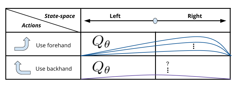
We'll borrow the example from the Udacity Nanodegree [8] to explain this issue a bit further: Suppose you are learning to play tennis and you are using the action-value function approximation algorithm from last section to learn from your tennis training experiences whether to use your forehand or backhand shots in specific situations. Recall that, unlike the tabular case, nearby pairs in state-action space will have similar values (which is actually what we wanted when discussing "generalization"). In the case of our tennis example, if we learn online as we practice we might start getting a situation that favors using our forehand shot (because we might have started getting more chances to use our forehand), which might be good for balls coming from the right. However, due to our function approximator, our Q-function will start to favor ever so slightly the forehand action even in cases were the ball comes to our left. I placed a question mark for the q-values of the other action as we might not know how their values are evolving as we update only the other action. If we have a single model for our \( Q_{\theta} \), as we change the weights of our network we will also slightly alter the values for other actions in potentially undesired ways.

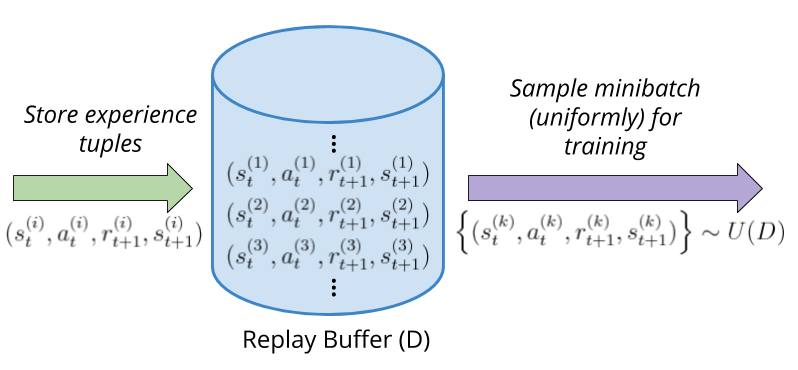
To solve these issues, the Experience Replay mechanism makes the agent learn from minibatches of past stored experience during training steps. We basically put all our experience in memory and then sample uniformly at random from it, which helps break the correlations between samples in the minibatch as they might not come from consequent steps (or even come from different episodes). This is depicted in Figure 13 below.

3.5.3 DQN: Fixed Targets

During training we are using the TD-target as the estimate of the true q-values that our Q-network should output for a specific pair \( (s,a) \) (as shown in the equation below). Unfortunately, this estimate is being computed using the current parameters of the Q-network which effectively is forcing us to follow a moving target. Besides, this is not mathematically correct, as we assumed these "true q-values" were not dependent on \( \theta \) (recall we did not take the gradient of this term).

\[ \theta := \theta + \alpha ( \overbrace{r + \max_{a'}Q(s',a';\theta)}^{\text{Computed with $\theta$}} - Q(s,a;\theta) ) \overbrace{\nabla_{\theta}Q_{\theta}\vert_{(s,a)}}^{\text{Computed with $\theta$}} \]

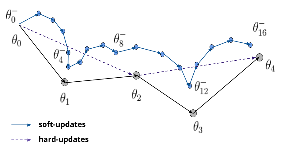
To help training stability the authors of [2] introduced the use of a separate network to compute these targets called a Target Network, which is almost the same as the network used for taking actions. The key difference is that the weights of this network are only copied from the weights of the other network after some specific number of steps. Therefore, the update rule can be modified as follows :

\[ \theta := \theta + \alpha ( \overbrace{r + \max_{a'}\underbrace{Q(s',a';\theta^{-})}_{\text{Target-network}}}^{\text{Computed with $\theta^{-}$}} - Q(s,a;\theta) ) \overbrace{\nabla_{\theta}Q_{\theta}\vert_{(s,a)}}^{\text{Computed with $\theta$}} \]

A slight variation to this update at constant intervals is to do updates every time step using interpolations, as shown in the following equation :

\[ \theta^{-} := (1 - \tau) \theta^{-} + \tau \theta \]

This are called soft-updates, and by adjusting the factor \( \tau \) (to some small values) we get a similar effect of copying the weights of the networks after a fixed number of steps. The difference is that, as the name suggests, these updates are less jumpy than the hard-updates made by copying entirely the weights of the network. At convergence, this update is very similar to a hard-update as the network weights do not change too much.

3.5.4 Sidenote: on the intuition behind issues with correlations

A way I like to use to reason about these issues related to correlations is by looking at the loss function we want to optimize (shown below). As you can see, we are computing a Mean-Square loss which computes the expectation over samples of the square differences between targets and current estimates.

\[ L({\theta}) = \mathbb{E}_{(s,a,r,s') \sim D} \left \{ ( r + \gamma \max_{a'} Q_{\theta}(s',a') - Q_{\theta}(s,a) )^{2} \right \} \]

As you can see, if our inputs (experience tuples) are correlated (breaking the i.i.d. assumption) we will not be able to compute this expectation from samples (can't apply the law of large numbers nor use a monte carlo estimate). Moreover, if trying to convert our RL problem into a supervised setting we will run into the issue that the target estimates (labels) should be decoupled from the estimates of our model. If not, we can run in instabilities by following a moving target, kind of like following our own opinions as universal truth, even when they might not be correct. Even more, if we start having strong opinions about a topic and use this to infer even more knowledge that reinforces these opinions, we will then fall into a vicious cycle of unstable learning. If that is the case in life, keep an open mind, recall good and bad experiences and don't forget to live with a little bit of \( \epsilon \) here and there 😉.

3.5.4 DQN: Putting it all together

Finally, by integrating all the previous improvements (Experience replay and Fixed targets) we get the complete version of the DQN algorithm from [2]. Below we show a modified version of the algorithm from [2] that uses soft-udpates instead of regular updates.

Deep-Q Learning with Experience Replay and Soft updates

• Initialize action-value function \( Q \) with parameters \( \theta \)
• Initialize target action-value function \( \hat Q \) with parameters \( \theta^{-} = \theta \)

• Initialize replay memory \( D \) to a certain capacity

• For \(episode = 0,1,2, \dots \)

  • Sample initial state \( s_{0} \) from the starting distribution
  • Preprocess: \( \phi_{0} = \phi( s_{0} ) \)
  • For \( t = 0,1,2, \dots \)
    • Select \( a_{t} \) from \( \phi_{t} \) using e-greedy from \( Q_{\theta} \)
    • Execute action \( a_{t} \) in the environment, and receive reward \( r_{t+1} \) and next state \( s_{t+1} \)
    • Preprocess: \( \phi_{t+1} = \phi( s_{t+1} ) \)
    • Store transition in replay buffer: \( (\phi_{t},a_{t},r_{t+1},\phi_{t+1}) \rightarrow D \)
    • Every \( T \) steps (training session):
      • Sample a minibatch \(\left \{ (\phi_{j}, a_{j}, r_{j+1}, \phi_{j+1}) \right \} \sim D \)
      • Set Q-targets: \(\\ y_{j} = \begin{cases} r_{j+1} &\text{if } s_{j+1} \text{ is terminal} \\ r_{j+1} + \gamma \max_{a'} \hat Q(\phi_{j+1},a';\theta^{-}) &\text{otherwise} \end{cases}\)
      • Update the action-value network parameters \( \theta \) by taking a step of SGD on \( (y_{j} - Q(\phi_{j},a_{j};\theta))^{2} \)
    • Update the target action-value network parameters \( \theta^{-} \) using soft updates: \(\\ \theta^{-} = (1-\alpha)\theta^{-} + \alpha \theta \)
  • Anneal \( \epsilon \) using a specified schedule

Below are some key aspects to take into consideration:

Preprocessing \( \phi_{t} = \phi( s_{t} ) \):

This step consists in converting the states|observations \( s_{t} \) received from the simulator into an appropriate state representation that can be used by our action-value network \( Q(\phi_{t},a_{t};\theta) \). We usually receive observations from the environment which in some cases (if we are lucky) consist of the actual internal state representation of the world. Unfortunately, in most cases we only receive observations that do not permit to fully recover the internal state of the environment. To avoid this issue we can design a state representation from these observations that would push us a bit more into the MDP setting and not the POMDP setting (Partially Observable MDP). In [2] the authors designed a state representation from the raw frame observations from the simulator by stacking a group of 4 consecutive frames, which tries to help encode a bit of temporal information (like speed and movement in the scene). This step is problem specific, and in our Banana collector case we chose to use the direct observations as state representation, although we could have made modifications to add more temporal information which could help with the problem of state aliasing. For further information on this topic you can watch part of this lecture from [7].

Grounding terminal estimates :

Grounding the estimates for terminal states is important because we don't want to make an estimate to the value for a terminal state bigger than what it could actually be. If we are just one step away of a terminal state, then our trajectories have length one and the return we obtain is actually only that reward. All previous algorithms do a check of whether or not a state is terminal in order to compute the appropriate TD-target. However, in tabular Q-learning you will find that in some implementations (unlike the one we presented earlier) there is no check similar to this one, but instead the entries of the Q-table are set to zeros for the terminal states, which is effectively the same as doing this check, as shown in the equation below:

\[ TD_{target} = r + \gamma \max_{a'}Q(s_{terminal}^{'},a') = r + \gamma max_{a'}0_{\vert \mathbb{A} \vert} = r \]

Unfortunaly, because we are dealing with function approximation, the estimates for a terminal states if evaluated will not return always zero, even if we initialize the function approximator to output zeros everywhere (like initializing the weights of a neural network to all zeros). This is caused by the fact that changes in the approximator parameters will affect the values of nearby states-action pairs in state-action space as well even in the slightest. For further information, you could check this lecture by Volodymyr Mnih from [9]. So, keep this in mind when implementing your own version of DQN, as you might run into subtle bugs in your implementations.

Exploration schedule :

Another important detail to keep in mind is the amount of exploration allowed by our \( \epsilon \)-greedy mechanism, and how we reduce it as learning progresses. This aspect is not only important in this context of function approximation, but in general as it's a key tradeoff to take into account (exploration v.s. exploitation dilemma). They idea is to give the agent a big enough number of steps to explore and get experiences that actually land some diverse good and bad returns, and then start reducing this ammount of exploration as learning progresses towards convergence. The mechanism used in [2] is to linearly decay \( \epsilon = 1.0 \rightarrow 0.1 \). Another method would be to decay it exponentially by multiplying \( \epsilon \) with a constant decay factor every episode. For further information you could check this lecture by David Silver from [6].

Choice for \( Q_{\theta}(s,a) \)

The last detail is related to the actual choice we make how to model our Q-network. We have two choices: either treat both inputs \( s,a \) as a single input \( (s,a) \) to the network, which would allows us to compute one q-value for a given state-action pair, or use \( s \) as only input to the network and grab all the q-values for all actions \( a \in \mathbb{A} \). Both of these options are shown in the figure below.

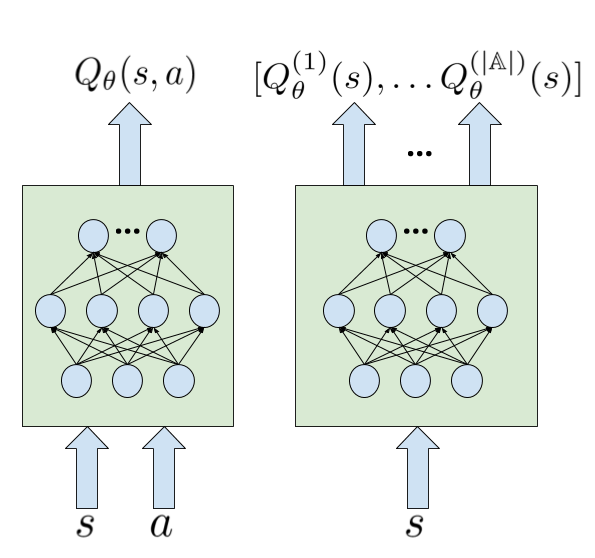
The first option would cost more as we need to compute all q-values in order to grab the maximum of them for both the TD-target calculation and the \( \epsilon \)-greedy action selection. The second option was the one used in [2], and it's the one will use for our implementation.

Sidenote : I couldn't help but notice that the cost function would change a bit due to our choice. Recall the loss function we defined for action-value function approximation:

\[ L(\theta) = \mathbb{E}_{s,a} \left \{ ( Q^{\star}(s,a) - \hat Q_{\theta}(s,a) )^{2} \right \} \]

If we use the network we chose before we would have to change the term \(\hat Q_{\theta}(s,a)\) by the term \(\hat Q_{\theta}^{(a)}(s)\) (or equivalently \(e_{a}^{T} \hat Q_{\theta}(s)\) if you prefer dot products). Thus, our loss function would change to:

\[ L(\theta) = \mathbb{E}_{s,a} \left \{ ( Q^{\star}(s,a) - \hat Q_{\theta}^{(a)}(s) )^{2} \right \} \]

Now, if we compute the gradient of this objective w.r.t. \( \theta \), after some operations (like in the function approximation derivation from earlier) we would get the following:

\[ \nabla_{\theta}L = \mathbb{E}_{s,a} \left \{ 2 ( Q^{\star}(s,a) - \hat Q_{\theta}^{(a)}(s) ) \nabla_{\theta} \hat Q_{\theta}^{(a)}(s) \right \} \]

Or, if using the dot product instead of indexing:

\[ \nabla_{\theta}L = \mathbb{E}_{s,a} \left \{ 2 ( Q^{\star}(s,a) - e_{a}^{T}\hat Q_{\theta}(s) ) \nabla_{\theta} (e_{a}^{T}\hat Q_{\theta}(s)) \right \} \]

If you expand the later (the gradient of the dot product) you can actually take that constant vector out, and then we would end up with the Jacobian of \( \hat Q_{\theta}(s) \). Both are at the end equivalent if you do the algebra, but I wonder how these are implemented by the autodiff. The funny thing is that this was a kind of hidden detail from most resources I found online. So, at first it looks like a linear regression problem (and that's how it should be if we had used the first option for the network instead), but instead it's like a multi-dimensional regression problem but with masks over some dimensions. Hopefully, autodiff handles this subtleties for us 😄. I'll update this part once I have some more time to get into the inner workings of the autodiff (so far, I was checking the torch's derivatives.yaml file where the gradient definitions are and it seems that the one doing the job might be the index_select_backward function when used by the kthvalue function, or the function index_select, or the function gather).

References

• [1] Sutton, Richard & Barto, Andrew. Reinforcement Learning: An introduction.
• [2] Mnih, Volodymyr & Kavukcuoglu, Koray & Silver, David, et. al.. Human-level control through deep-reinforcement learning
• [3] Achiam, Josh. Spinning Up in Deep RL
• [4] Simonini, Thomas. A Free course in Deep Reinforcement Learning from beginner to expert
• [5] Stanford RL course by Emma Brunskill
• [6] UCL RL course, by David Silver
• [7] UC Berkeley DeepRL course by Sergey Levine
• [8] Udacity DeepRL Nanodegree
• [9] DeepRL bootcamp
• [10] Van Hasselt, Hado. Double Q-learning
• [11] Van Hasselt, Hado & Guez, Arthur & Silver, David. Deep Reinforccement Learning with Double Q-learning
• [12] Schaul, Tom & Quan, John & Antonoglou, Ioannis & Silver, David. Prioritized Experience Replay
• [13] Hacker Earth. Segment Trees data structures
• [14] OpenAI. Baselines
• [15] Hessel, Matteo & Modayil, Joseph & van Hasselt, Hado & Schaul, Tom & Ostrovski, Georg & Dabney, Will & Horgan, Dan & Piot, Bilal & Azar, Mohammad & Silver, David Rainbow
• [16] Hausknecht, Matthew & Stone, Peter Deep Recurrent Q-Learning with Partially Observable MDPs