Udacity DeepRL project 1: Navigation - Part (3⁄3)
Using DQN to solve the Banana environment from ML-Agents
This is an Part-3 of an accompanying post for the submission of the Project 1: navigation from the Udacity Deep Reinforcement Learning Nanodegree, which consisted on building a DQN-based agent to navigate and collect bananas from the Banana Collector environment from Unity ML-Agents.

The following are the topics to be covered in this post:
- An overview of the improvements to vanilla DQN
- Some preliminary tests of the improvements
- Final remarks and future improvements
7. An overview of the improvements to vanilla DQN
After completing the base DQN implementation I decided to try implementing the improvements mentioned in the lectures, namely: Double DQN, Prioritized Experience Replay, and Dueling DQN. So far, we have implemented the first two, and in this section we will discuss them both.
7.1 Double DQN
This improvement tries to deal with the overestimation of the action-values that are used for the TD-targets. Recall the targets calculation from vanilla DQN:
\[ TD_{targets} = r + \gamma \max_{a'}Q(s',a';\theta^{-}) \]
By definition, we can rewrite this equation as follows :
\[ TD_{targets} = r + \gamma Q(s',\argmax_{a'}Q(s',a';\theta^{-});\theta^{-}) \]
These two eqs. are equivalent because we are evaluating the Q-value for the greedy action (second eq.), which is the same as taking the max. Q-value over all actions (first eq.). Let's make the components of the equation even clearer, by identifying each term:
\[ TD_{targets} = r + \gamma \underbrace{Q(s',\overbrace{\argmax_{a'}Q(s',a';\theta^{-})}^{\text{Action chosen to be the best}};\theta^{-})}_{q_{best}:\text{Q-value for the "best" action}} \]
The issue with this evaluation comes from evaluating q-values for actions chosen to be the best in specific steps during training, which might not be the best. Also even if these actions are actually the best actions, we still could overestimate its value because the network that evaluates it might just not be fully trained properly (which happens in early stages of training).
To avoid this issue of overestimation the authors of [11] introduced the idea of Double DQN, which builds on top of the idea of Double Q-learning introduced by Van Hasselt [10]. The idea consists of using two function approximators to compute the TD-targets, instead of just one, as shown in the following equation.
\[ TD_{targets} = r + \gamma \underbrace{Q(s',\overbrace{\argmax_{a'}Q(s',a';\theta)}^{\text{Chosen using $Q_{\theta}$}};\theta^{-})}_{\text{Evaluated using $Q_{\theta^{-}}$}} \]
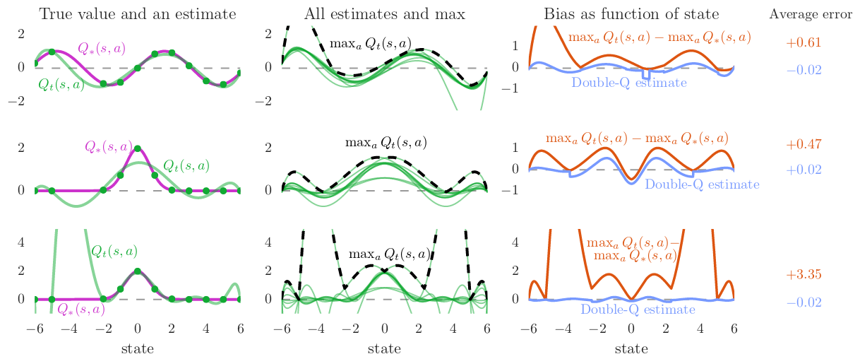
Some visualizations from [11] are shown below, which show the effect of overestimation when using function approximation (in a simple test problem) and how Double Q-learning can potentially fix these issues. The test problem consists on a continuous state-space with just 1 dimension (shown along x-axis) and a discrete action space with 10 actions. The problem is set up such that all actions have the same true value equal to the optimal value ( \( Q^{\star}(s,a) = V^{\star}(s), \forall a \in \mathbb{A} \) ). The estimates are built using polinomials of 6th degree fitted to samples of the optimal Q-value function at various points of the state space. Rows represent cases with different \( Q^{\star} \), whereas columns represent the study of overestimation.
As suggested in [11], the easiest addition we can make to our code is to use both action-value and target action-value networks for Double DQN, using the action-value network for computing the greedy action, and the target network to evalue the q-value for this action. A snippet of these changes (from the agent.py file) that implements the required steps is shown below:
if self._useDoubleDqn :
    # targets are computed in the following way
    #
    #
    # q-target = r + gamma * Q( s', argmax( Q(s',a';theta) ); theta )
    #                        ^         a'               actor     target
    #                        |
    #                        |              ^
    #     qvalue from target model          |
    #                                       |
    #                             greedy action from actor model

    # compute qvalues from both actorModel and targetModel
    _qvals_actorModel_s   = self._qmodel_actor.eval( _nextStates )
    _qvals_targetModel_s  = self._qmodel_target.eval( _nextStates )

    # greedy actions
    _argmaxActions = np.argmax( _qvals_actorModel_s, 1 ).reshape( -1, 1 )

    # compute qtargets from the qvals of target network, ...
    # using greedy actions from the actor network
    _qtargets = _rewards + ( 1 - _dones ) * self._gamma * \
                np.squeeze( np.take_along_axis( _qvals_targetModel_s, _argmaxActions, axis = 1 ) )
else :
    # targets are just computing the target network
    _qtargets = _rewards + ( 1 - _dones ) * self._gamma * \
                np.max( self._qmodel_target.eval( _nextStates ), 1 )
7.2 Prioritized Experience Replay
So far we have been sampling uniformly from the replay buffer, regardless of how important the experience tuples might be for training, which seems not intuitive as during our experiences with the world there might be some experiences that could help us learn the most (kind of life lessons). Prioritized Experience Replay (PER), introduced in [12], is a heuristic that tries to solve this problem by adding some priority to certain experience tuples in the replay buffer, and then sample them according to these priorities.
So, instead of sampling uniformly from the replay buffer:
\[ \left \{ ( s_{j}, a_{j}, r_{j+1}, a_{j+1} ) \right \} \sim D_{vanilla} \]
PER samples in a prioritized way from the replay buffer:
\[ \left \{ ( s_{j}, a_{j}, r_{j+1}, a_{j+1}, w_{j} ) \right \} \sim D_{prioritized} \]
There are various details that have to be considered in order to implement PER, namely:
- What measure should we use for the priorities?
- Why is there a \( w_{j} \) in the returned samples?
- How do we add priorities to the replay buffer, and how do we sample?
These details are related to (respectively):
- Computing priorities from Bellman Errors.
- Importance Sampling (we have to fix a distribution mismatch).
- An efficient implementation for the prioritized buffer.
Computing priorities
The measure we will use to compute priorities are the Bellman Errors (or TD-Errors), whose expression is shown below (without the double dqn improvement):
\[ \delta = r + \gamma \max_{a'} Q(s',a';\theta^{-}) - Q(s,a;\theta) \]
This makes sense as a measurement because if the errors are big, then that is a measure of how off are our estimates. For the case that we had an oracle (true q-values for the targets), these errors are the actual values we have to be close to. In our case, we are using estimates with the target network, but these still give some similar information. Moreover, the targets at almost terminal states (1-step before terminal) reduce to the actual returns from those states, so if they are in the replay buffer, and the error is big for them, we should use them with more priority. So, we have the following measure for our priorities, using the absolute value of the Bellman Error:
\[ p_{t} = \vert \delta_{t} \vert \]
Thus, we can sample using this priorities by defining the following probability for each sample:
\[ P(j) = \frac{p_{j}}{\sum_{k}p_{k}} \]
A slight issue comes when the TD-error is very small (or even zero). This makes the sampling process avoid picking experiences that have small TD-error (or even not picking them at all if zero). So, to avoid this issue a small positive amount of priority is added to ensure the priorities don't become zero, as shown in the equation below.
\[ p_{t} = \vert \delta_{t} \vert + e \]
Finally, to control how much we let the priority affect the sample probabilities a hyperparameter \( \alpha \) is introduced as follows:
\[ P(j) = \frac{p_{j}^{\alpha}}{\sum_{k}p_{k}^{\alpha}} \]
Sampling from a different distribution
Because we are sampling using the priorities, we are effectively sampling from another distribution (other than the uniform distribution). Notice that the priorities will make some samples come more frequently than others. Also, try to visualize how the distribution changes from uniform to a distribution with peaks that depend on the priorities.
Recall our objective, which was defined as an expectation:
\[ L(\theta) = \mathbb{E}_{(s,a,r,s') \sim D} \left \{ ( r + \gamma \max_{a'} Q_{\theta^{-}}(s',a') - Q_{\theta}(s,a) )^{2} \right \} \]
To effectively remove the mismatch in distributions we have to make use of Importance Sampling as follows:
\[ L(\theta) = \mathbb{E}_{(s,a,r,s') \sim D_{prioritized} } \left \{ \frac{p(D)}{p(D_{prioritized})} ( r + \gamma \max_{a'} Q_{\theta^{-}}(s',a') - Q_{\theta}(s,a) )^{2} \right \} \]
The ratio \( w = \frac{p(D)}{p(D_{prioritized})} \) is the weight that has to be applied to correct for this mismatch, and it's computed from the probability that a sample is drawn from the buffer uniformly \( p(D) \), and the probability that a sample is drawn from the buffer using priorities \( p(D_{prioritized}) \). These weights can then be used to compute a modified loss function. As we will see in the implementation section later, instead of directly using the Mean Square Error loss from our DL package, we will make a modified loss to take into account importance sampling weights.
Data structure for sampling and storing with priorities
For the replay buffer from vanilla DQN we used a simple deque (or we could have also use a big numpy array an keep track of a buffer indexing variable). To support sampling using priorities the authors of [12] give two possible implementations (see Appendix B.2.1 from [12]):
- Rank-based prioritization: This implementation makes use of a priority queue built using a binary heap.
- Proportional prioritization: This implementation uses a "sum-tree" data structure.
We will use the second implementation, and explain how the datastructure works to enable efficient storing and sampling using priorities. This makes use of a Sum Tree, which is a specific case of a Segment Tree data structure, which consists of (quoting the previous linked resource):
"A Segment Tree is basically a binary tree used for storing intervals or segments. Each node in the segment Tree represents an interval"
An example of a Segment Tree is shown below:
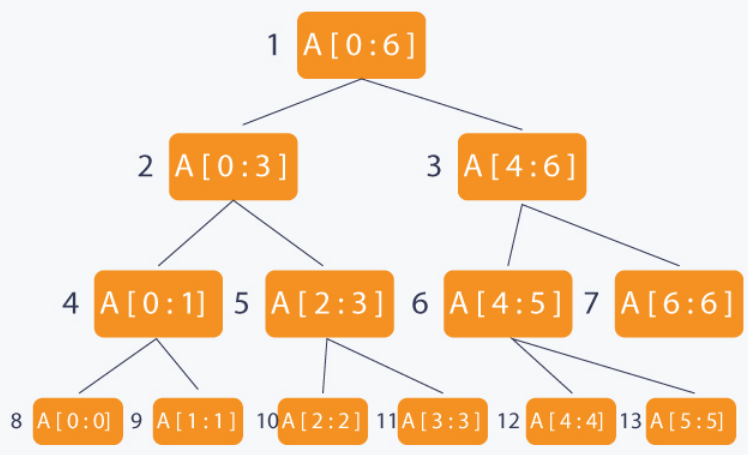
As you can see from the figure, each node in the tree represents an interval. Because it's a binary tree, we can efficiently query and update specific interval in O(log n), and worst case O(n) if the tree is unbalanced.
We can make use of this property of querying intervals to make efficient samples using priorities, where each interval at the leaves would consist of the priorities each leave has. The Segment Tree used for this case is a Sum Tree, which implements a Segment Tree with a sum operator that stores in each node the sum of its children. An example of such sum tree is shown below :
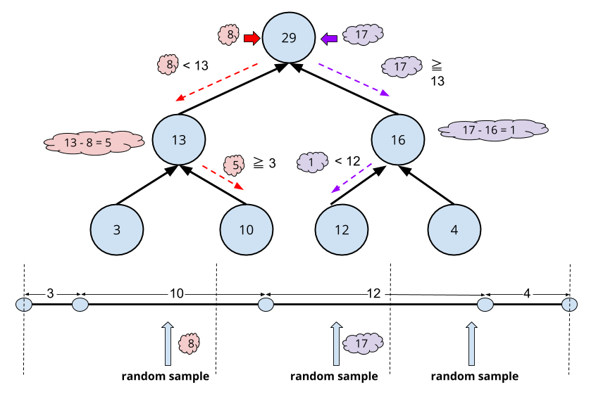
From the figure we could also see that in order to sample using the priorities in the leaves of the tree we essentially divide the whole segment composed of the unions of the priorities as segments into a number of bins required by the number of samples that we want to take (3 in that case). This effectivetly let's us sample using the priorities because each priority becomes a segment, and the chance of a random sample in a bin to land in that segment is proportional to the length of the segment.
The Sum Tree let's us query in which interval a given random number will land, by searching through the nodes of the tree until the required leave is found (corresponding to the interval in which the sample will land in the union of segments view).
Finally, updates can also be made to the tree when new priorities are available, i.e. when new bellman errors are computed for a minibatch. Notice that we are updating priorities over the minibatch only, and not the whole elements in the prioritized replay buffer, which is discussed in section 3.3 on Stochastic Prioritization in [12].
Implementation
The full implementation of PER is distributed over four files:
segmentree.py, which implements the Segment Tree, Sum Tree, and Min Tree (used for keeping track of the min priority) data structures. This implementation was based on OpenAI baselines [14], and in this and this two implementations. We kept a MinTree as in the OpenAI baselines implementation to be consistent with their implementation. However, I think we could have just kept a variable updated with the min at each update of the priorities as well.
prioritybuffer.py, which implements the prioritized replay buffer. It was also based on the three resources mentioned above.
agent.py, which has a slight modification for the learning method to take into account importance sampling.
model_pytorch.py, which implements the required modifications to the loss function when using PER.
We will focus mainly in the implementation of the priority buffer, the changes made to the agent base code and the changes made to the model. I'd suggest the reader to refer to the resources about the segmentree and the implementation (this one and the others as well) to fully understand the sumtree and mintree data structures. Some tests of the segmentTree, sumTree and minTree can be found in the tests.ipynb notebook at the root of the provided package.
The key methods in the priority buffer are the __init__ add, sample and updatePriorities methods, which we will analyze one by one.
- The constructor ( __init__ ) instantiates the prioritized replay buffer by copying the required hyperparameters, namely: \( e \) extra amount for priority (recall \( p_{t} = \vert \delta_{t} \vert + e \) ), \( \alpha \) power to control how priority affects the sample probability, \( \beta \) power to control the amount of importance sampling used (annealed from given value up to 1), and the amount \( \Delta \beta \) that the \( \beta \) factor increases every sampling call. We also create the Sum Tree and the Min Tree as required for the sampling and importance sampling calculation process.
    def __init__( self,
                  bufferSize,
                  randomSeed,
                  eps = 0.01,
                  alpha = 0.6,
                  beta = 0.4,
                  dbeta = 0.00001 ) :

        super( DqnPriorityBuffer, self ).__init__( bufferSize, randomSeed )

        # hyperparameters of Prioritized experience replay
        self._eps   = eps    # extra ammount added to the abs(tderror) to avoid zero probs.
        self._alpha = alpha  # regulates how much the priority affects the probs of sampling
        self._beta  = beta   # regulates how much away from true importance sampling we go (up annealed to 1)
        self._dbeta = dbeta  # regulates how much we anneal up the previous regulator of importance sampling

        # a handy experience tuple constructor
        self._experience = namedtuple( 'Step',
                                       field_names = [ 'state',
                                                       'action',
                                                       'reward',
                                                       'nextState',
                                                       'endFlag' ] )
        # sumtree for taking the appropriate samples
        self._sumtree = segmentree.SumTree( self._bufferSize )
        # mintree for taking the actual min as we go
        self._mintree = segmentree.MinTree( self._bufferSize )

        # a variable to store the running max priority
        self._maxpriority = 1.
        # a variable to store the running min priority
        self._minpriority = eps

        # number of "actual" elements in the buffer
        self._count = 0
- The add method adds an experience tuple to the buffer. We create the experience object (data of the leaves of the trees), and add it to both the Sum Tree and the Min Tree with maximum priority (as we want to make sure new experiences have a better chance of being picked at least once).
    def add( self, state, action, nextState, reward, endFlag ) :
        """Adds an experience tuple to memory

        Args:
            state (np.ndarray)      : state of the environment at time (t)
            action (int)            : action taken at time (t)
            nextState (np.ndarray)  : state of the environment at time (t+1) after taking action
            reward (float)          : reward at time (t+1) for this transition
            endFlag (bool)          : flag that indicates if this state (t+1) is terminal

        """

        # create a experience object from the arguments
        _expObj = self._experience( state, action, reward, nextState, endFlag )

        # store the data into a node in the smtree, with nodevalue equal its priority
        # maxpriority is used here, to ensure these tuples can be sampled later
        self._sumtree.add( _expObj, self._maxpriority ** self._alpha )
        self._mintree.add( _expObj, self._maxpriority ** self._alpha )

        # update actual number of elements
        self._count = min( self._count + 1, self._bufferSize )
- The sample method is the most important one, as it is in charge of sampling using the Sum Tree and computing the importance sampling weights using both the Sum Tree and Min Tree. As explained earlier, the sampling process consists of sampling random numbers inside bins over the whole union of priorities by querying the Sum Tree with these random numbers. The importance sampling weights are computed as explained earlier, and returned along the corresponding experience tuple for usage in the SGD process during learning. We also return the indices in the tree that correspond to these samples for later updates, as the Bellman Errors will be computed for these experiences and updated after the SGD step has been taken (shown later in the modifications to the core agent functionality).
    def sample( self, batchSize ) :
        """Samples a batch of data using consecutive sampling intervals over the sumtree ranges

        Args:
            batchSize (int) : number of experience tuples to grab from memory

        Returns:
            (indices, experiences) : a tuple of indices (for later updates) and
                                     experiences from memory

        Example:

                    29
                   /  \
                  /    \
                 13     16
                |  |   |  |
               3  10  12  4       |---| |----------| |------------| |----|
                                    3        10            12          4
                                  ^______^______^_______^_______^_______^
                                        *      *      *   *    *     *

            5 samples using intervals, and got 10, 10, 12, 12, 4
        """
        # experiences sampled, indices and importance sampling weights
        _expBatch = []
        _indicesBatch = []
        _impSampWeightsBatch = []

        # compute intervals sizes for sampling
        _prioritySegSize = self._sumtree.sum() / batchSize

        # min node-value (priority) in sumtree
        _minPriority = self._mintree.min()
        # min probability that a node can have
        _minProb = _minPriority / self._sumtree.sum()

        # take sampls using segments over the total range of the sumtree
        for i in range( batchSize ) :
            # left and right ticks of the segments
            _a = _prioritySegSize * i
            _b = _prioritySegSize * ( i + 1 )
            ## _b = min( _prioritySegSize * ( i + 1 ), self._sumtree.sum() - 1e-5 )

            # throw the dice over this segment
            _v = np.random.uniform( _a, _b )
            _indx, _priority, _exp = self._sumtree.getNode( _v )

            # Recall how importance sampling weight is computed (from paper)
            #
            # E   { r } = E    { p * r  } = E     { w * r }  -> w : importance
            #  r~p         r~p'  -           r~p'                   sampling
            #                    p'                                 weight
            #
            # in our case:
            #  p  -> uniform distribution
            #  p' -> distribution induced by the priorities
            #
            #      1 / N
            #  w = ____
            #
            #       P(i) -> given by sumtree (priority / total)
            #
            # for stability, the authors scale the weight by the max-weight ...
            # possible, which is (because maximizing a fraction minimizes the ...
            # denominator if the numrerator is constant=1/N) the weight of the ...
            # node with minimum probability. After some operations :
            #
            #                          b                     b
            # w / wmax = ((1/N) / P(i))   / ((1/N) / minP(j))
            #                                          j
            #                               b                      -b
            # w / wmax = ( min P(j) / P(i) )   = ( P(i) / min P(j) )
            #               j                              j

            # compute importance sampling weights
            _prob = _priority / self._sumtree.sum()
            _impSampWeight = ( _prob / _minProb ) ** -self._beta

            # accumulate in batch
            _expBatch.append( _exp )
            _indicesBatch.append( _indx )
            _impSampWeightsBatch.append( _impSampWeight )

        # stack each experience component along batch axis
        _states = np.stack( [ exp.state for exp in _expBatch if exp is not None ] )
        _actions = np.stack( [ exp.action for exp in _expBatch if exp is not None ] )
        _rewards = np.stack( [ exp.reward for exp in _expBatch if exp is not None ] )
        _nextStates = np.stack( [ exp.nextState for exp in _expBatch if exp is not None ] )
        _endFlags = np.stack( [ exp.endFlag for exp in _expBatch if exp is not None ] ).astype( np.uint8 )

        # convert indices and importance sampling weights to numpy-friendly data
        _indicesBatch = np.array( _indicesBatch ).astype( np.int64 )
        _impSampWeightsBatch = np.array( _impSampWeightsBatch ).astype( np.float32 )

        # anneal the beta parameter
        self._beta = min( 1., self._beta + self._dbeta )

        return _states, _actions, _nextStates, _rewards, _endFlags, _indicesBatch, _impSampWeightsBatch
- The updatePriorities method is in charge of updating the priorities of the sampled experiences using the new Bellman Errors computed during the SGD learning step.
    def updatePriorities( self, indices, absBellmanErrors ) :
        """Updates the priorities (node-values) of the sumtree with new bellman-errors

        Args:
            indices (np.ndarray)        : indices in the sumtree that have to be updated
            bellmanErrors (np.ndarray)  : bellman errors to be used for new priorities

        """
        # sanity-check: indices bath and bellmanErrors batch should be same length
        assert ( len( indices ) == len( absBellmanErrors ) ), \
               'ERROR> indices and bellman-errors batch must have same size'

        # add the 'e' term to avoid 0s
        _priorities = np.power( absBellmanErrors + self._eps, self._alpha )

        for i in range( len( indices ) ) :
            # update each node in the sumtree and mintree
            self._sumtree.update( indices[i], _priorities[i] )
            self._mintree.update( indices[i], _priorities[i] )
            # update the max priority
            self._maxpriority = max( _priorities[i], self._maxpriority )
The key changes made to the agent core functionality are located in the learn method.
- We first just sample using the priority buffer, which returns also the importance sampling weights to be use later in the SGD step (see line 221).
        # get a minibatch from the replay buffer
        _minibatch = self._rbuffer.sample( self._minibatchSize )
        if self._usePrioritizedExpReplay :
            _states, _actions, _nextStates, _rewards, _dones, _indices, _impSampWeights = _minibatch
        else :
            _states, _actions, _nextStates, _rewards, _dones = _minibatch
- We then just execute the training step on the action-value network as usual, with the slight addition of the importance sampling weights. After this step, we grab the Bellman Errors computed inside the model's functionality and use them to update the priorities of the sampled experiences in the minibatch (see line 277).
        # make the learning call to the model (kind of like supervised setting)
        if self._usePrioritizedExpReplay :
            ## if np.sum( _rewards ) > 0. :
            ##     set_trace()
            # train using also importance sampling weights
            _absBellmanErrors = self._qmodel_actor.train( _states, _actions, _qtargets, _impSampWeights )
            # and update the priorities using the new bellman erros
            self._rbuffer.updatePriorities( _indices, _absBellmanErrors )
        else :
            # train using the normal data required
            self._qmodel_actor.train( _states, _actions, _qtargets )
Finally, the key changes made to the model are located in the initialize and train methods:
- The initialize method constructs the appropriate loss function for the case of using importance sampling (for PER) by making a custom MSE loss that includes the weights coming from importance sampling.
    def initialize( self, args ) :
        # grab current pytorch device
        self._device = args['device']
        # send network to device
        self._nnetwork.to( self._device )
        # create train functionality if necessary
        if self._trainable :
            # check whether or not using importance sampling
            if self._useImpSampling :
                self._lossFcn = lambda yhat, y, w : torch.mean( w * ( ( y - yhat ) ** 2 ) )
            else :
                self._lossFcn = nn.MSELoss()
            self._optimizer = optim.Adam( self._nnetwork.parameters(), lr = self._lr )
- The train method takes into account the use of importance sampling by passing the importance sampling weights to an appropriate tensor and then calling the appropriate loss function. The bellman errors are computed by default (as we are saving them), but are only grabbed by the agent if using PER.
    def train( self, states, actions, targets, impSampWeights = None ) :
        if not self._trainable :
            print( 'WARNING> tried training a non-trainable model' )
            return None
        else :
            _aa = torch.from_numpy( actions ).unsqueeze( 1 ).to( self._device )
            _xx = torch.from_numpy( states ).float().to( self._device )
            _yy = torch.from_numpy( targets ).float().unsqueeze( 1 ).to( self._device )

            # reset the gradients buffer
            self._optimizer.zero_grad()

            # do forward pass to compute q-target predictions
            _yyhat = self._nnetwork( _xx ).gather( 1, _aa )

            ## set_trace()

            # and compute loss and gradients
            if self._useImpSampling :
                assert ( impSampWeights is not None ), \
                       'ERROR> should have passed importance sampling weights'

                # convert importance sampling weights to tensor
                _ISWeights = torch.from_numpy( impSampWeights ).float().unsqueeze( 1 ).to( self._device )

                # make a custom mse loss weighted using the importance samples weights
                _loss = self._lossFcn( _yyhat, _yy, _ISWeights )
                _loss.backward()
            else :
                # do the normal loss computation and backward pass
                _loss = self._lossFcn( _yyhat, _yy )
                _loss.backward()

            # compute bellman errors (either for saving or for prioritized exp. replay)
            with torch.no_grad() :
                _absBellmanErrors = torch.abs( _yy - _yyhat ).cpu().numpy()

            # run optimizer to update the weights
            self._optimizer.step()

            # grab loss for later statistics
            self._losses.append( _loss.item() )

            if self._saveGradients :
                # grab gradients for later
                _params = list( self._nnetwork.parameters() )
                _gradients = [ _params[i].grad for i in range( len( _params ) ) ]
                self._gradients.append( _gradients )

            if self._saveBellmanErrors :
                self._bellmanErrors.append( _absBellmanErrors )

            return _absBellmanErrors
8. Some preliminary tests of the improvements
In this section we show some preleminary results obtained with the improvements. These results come from the following two extra experiments, which we made in order to evaluate if PER and DDQN helped during training:
- Experiment 2 : Test vanilla DQN against each of the improvements (DDQN only, PER only and DDQN + PER).
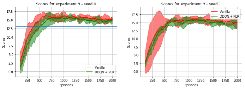
- Experiment 3 : Test if DDQN + PER help in situations with too little exploration. Our hypothesis was that too little exploration might run into unstable learning, and DDQN + PER could help stabilize this process (or even help solve it if the agent couldn't solve the task using only the baseline).
Note: the hyperparameters related to PER were not exposed through the .json file (sorry,I will fix it in later tests), but instead hard-coded in the priority-buffer implementation (see the prioritybuffer.py file). These parameters were set to the following default values:
eps   : 0.01    # small value added to the absolute value of the bellman error
alpha : 0.6     # power to raise the priority in order to further control it
beta  : 0.4     # importance sampling annealed factor
dbeta : 0.00001 # linear increment per sample added to the "beta" parameter
Spoiler alert: we did not find much improvement in the task at hand by using PER and DDQN. However, these results are preliminary as we did not tune the hyperparameters of PER (nor the other hyperparameters), and we still haven't made test cases for all details of the implementations of the algorithm. We tested each separate component of the improvements (extra data structures, consistency with other sources' implementations, etc.), but still we could have miss some detail in the implementation. Also, perhaps the structure of the task at hand is not too complicated for our vanilla DQN to require these improvements. We plan to make further tests and experiments in this and more complicated environments (visual banana environment, atari, etc.) to see if our improvements actually work and help during training.
8.1 Experiment 2: Testing DQN improvements against the baseline
This experiment consisted of testing what improvements do DDQN and PER offer to our vanilla DQN implementation. The configurations for these can be found in the following files:
- config_agent_2_1.json : Configuration with only DDQN active.
- config_agent_2_2.json : Configuration with only PER active.
- config_agent_2_3.json : Configuration with DDQN + PER active.
- config_agent_1_1.json : The baseline, with the same hyperparameters as the ones above.
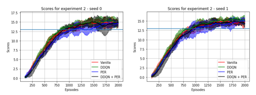
We used 5 runs and 2 different seeds for each configuration of the experiment. The preliminary results (shown below) look very similar for all configurations, and we can't conclude if there is any improvement using the variations to vanilla DQN.
8.2 Experiment 3: Testing DQN
This experiment consisted on testing if DDQN + PER would help in situations where there is too little exploration. The configurations used for these experiment can be found in the following files:
- config_agent_3_1.json : Configuration without DDQN nor PER.
- config_agent_3_2.json : Configuration with DDQN + PER active.
The exploration schedule was such that in just 60 episodes we would have reached the fixed 0.01 minimum value for \( \epsilon \), and have just 18000 experience tuples in a buffer of size of 131072, which consisted just of a approx. 13% of the replay buffer size. All other interactions would add only experience tuples taken from a practically greedy policy. Also, after just 510 episodes, the replay buffer would have just experience tuples sampled from a greedy policy.
We considered that this case would require clever use of the data (PER) to squeeze the most out of the experiences in the replay buffer, and also to not to overestimate the q-values, as we would be following a pure greedy policy after just some steps. The preliminary results don't show much evidence of improvement, except in a run with a different seed, in which the learning curves were less jumpy, indicating more stable learning. The results are shown in the image below, which were created using 5 runs with 2 seeds for both configurations.
9. Final remarks and future improvements
In this post we tried to explain the DQN algorithm and how to use it to solve the banana environment collector task from the ml-agents package. We also implemented some improvements to the base DQN implementation, namely DDQN and PER. Some conclusions we can get from this project would be the following:
Deep reinforcement learning via DQN is a very interesting approach to solve control problems. Not control as in continuous control (which is a subject very close to my heart 😄), as we are dealing with only discrete action spaces. However, as we will see in the following projects, this approach of end-to-end learning of behaviours can be scaled up to this environments that require continuous state and action spaces (so stay tuned for the DDPG and PPO post for project 2 😄).
The additions made to action-value function approximation by the DQN authors are quite important. We mentioned a case in which we messed up the soft-updates and were effectively copying the full networks from one to another at a very high frequency (every 4 steps, almost every single step). This is very similar to the case of just using a single network (so no effective target-network). In a sense we did an ablation test without realizing it 😄 (my bad). I'll make more proper ablation tests as I update this post, like removing fixed-targets and removing the replay-buffer.
We also did not mentioned it in a proper section, but we got some interesting behaviour while working with the project. In some situations the agent got stuck during testing, trying to go left and then right, stuck in an loop from which it could not recover (those are the spikes that appear in the noisy plots, which appear very sporadically). This behaviour is kind of similar to how a state-machine of a game agent gets stuck because the programmer forgot to take into account some detail of the game (I've been there quite some times 😢). For this situation I just made the MLP bigger (give it a bigger high capacity model) and it started getting better performance and got stuck less often, kind of like having more "if-then soft rules" to work with that help take into account those details. This could be also caused because various states of the environment are aliased, as we only have ray-casting observations feed to a MLP, so perhaps using a recurrent model would help in this situation.
Also, there's some unexpected behaviour that we can see when we look at the q-values visualizations during testing (see Figure 20). We expected to see a clear differences between the max. q-value and the other q-values, but instead we can just see a small margin that defines the actual action to choose. We haven't run the visualizer into other environments to see if there's a clear distinction during inference, and we consider that this might be caused by the nature of the environment (lunar-lander), as perhaps in a given state you can actually get the same reward if any action is taken, given that the next states will give you different situations that might yield to more distinct q-values (imagine starting taking a bad action, but your policy let's you recover, and in this situations you see a clear difference). We will try to further analyze this in future updates to the post.
Finally, below we mention some of the improvements we consider making in following updates to this post:
Make more tests of the improvements implemented, namely DDQN and PER, as we did not see much improvement in the given task. We could run the implementation in different environments from gym and atari, make "unit tests" for parts of the implementation, and tune the hyperparameters (PER) to see if there are any improvements.
Get the visual-based agent working for the banana environment. We had various issues with the executable provided, namely memory leaks of the executable that used up all memory in my machine. I first thought they were issues with the replay buffer being to big (as the experiences now stored images), but after some debugging that consisted on checking the system-monitor and even only testing the bare unity environment in the most simple setting possible, i.e. just instantiating it and running a random policy in a very simple script, we still got leaks that did not let us fully test our implementation. I was considering sending a PR, but the leaks only occur using the old ml-agent API (called unityagents, which is version 0.4.0). We made a custom build in the latest version of unity ml-agents and the unity editor, and got it working without leaks, but still could not get the agent to learn, which might be caused by our DQN agent implementation, our model, or the custom build we made.
Finish the implementation of a generic model for tensorflow and pytorch (see the incomplete implementations in the model_pytorch.py and model_tensorflow.py files), in order to be able to just send a configuration easily via a .json file or similar, and instantiate the requested model without having to write any pytorch nor tensorflow specific model by ourselves.
Implement the remaining improvements from rainbow, namely Dueling DQN, Noisy DQN, A3C, Distributional DQN, and try to reproduce a similar ablation test in benchmarks like gym and ml-agents.
Implement recurent versions of DQN and test the implementation in various environments.
References
- [1] Sutton, Richard & Barto, Andrew. Reinforcement Learning: An introduction.
- [2] Mnih, Volodymyr & Kavukcuoglu, Koray & Silver, David, et. al.. Human-level control through deep-reinforcement learning
- [3] Achiam, Josh. Spinning Up in Deep RL
- [4] Simonini, Thomas. A Free course in Deep Reinforcement Learning from beginner to expert
- [5] Stanford RL course by Emma Brunskill
- [6] UCL RL course, by David Silver
- [7] UC Berkeley DeepRL course by Sergey Levine
- [8] Udacity DeepRL Nanodegree
- [9] DeepRL bootcamp
- [10] Van Hasselt, Hado. Double Q-learning
- [11] Van Hasselt, Hado & Guez, Arthur & Silver, David. Deep Reinforccement Learning with Double Q-learning
- [12] Schaul, Tom & Quan, John & Antonoglou, Ioannis & Silver, David. Prioritized Experience Replay
- [13] Hacker Earth. Segment Trees data structures
- [14] OpenAI. Baselines
- [15] Hessel, Matteo & Modayil, Joseph & van Hasselt, Hado & Schaul, Tom & Ostrovski, Georg & Dabney, Will & Horgan, Dan & Piot, Bilal & Azar, Mohammad & Silver, David Rainbow
- [16] Hausknecht, Matthew & Stone, Peter Deep Recurrent Q-Learning with Partially Observable MDPs